Introduction

Species distributional patterns are neither stable nor random, and follow geographic patterns that reflect both recent ecological conditions and processes and phylo-geographic history (Avise 2000). At present time, species that originated in the past as small disjunct populations seem to have rearranged their current distributions showing a sympatric or parapatric assemblage in areas of high current capacity (Fjeldså 1995). Thus, present distribution of the Andean biota reflects today's biotic and abiotic interactions of the species and the ecosystems in which they occur. As a result, species distribution and accumulation in such areas seems to be related to a sharp replacement of different habitat types within short distances (Fjeldså et al. 1999; García-Moreno et al. 1999).

Because distribution patterns are not homogeneous, it is more likely to argue the presence of specific environmental conditions within the carrying capacity areas that favor species accumulation. According to Boone et al. (2000) the spatial heterogeneity observed at present in biotic communities is an expression of the biotic and abiotic factors that shape the n-dimensional space of the specie's niche (Hutchinson 1957). Subsequently, the spatial distribution of Andean centered taxa could be explained by the environmental gradients present on the Andean chain.

To understand patterns of species diversity, it is necessary to evaluate the temporal and spatial processes that have shaped their current distribution and the ones that sustain them at present time (Heindl & Schuchmann 1998; Huston 2002). Thus, generating detailed and accurate distributional information for such species becomes a critical step in such understanding process (Peterson et al. 2002).

Museum and herbarium specimens constitute the primary documentation of a species´ true presence records. However, information of species´ true absence is almost nonexistent. These drawbacks reflect on the production of species geographic ranges represented by simple collection point dots plotted over country base maps. In the best scenario species geographic ranges are presented as shaded outline maps that connects know collection localities (Anderson & Martínez-Meyer 2004).

A potential non-subjective approach to maximize the utility of available distribution data for such areas is to develop species-distribution models (SDMs). Recent advances employing geographic information systems (GIS) technology allow correlative modeling of species' potential macro-distributions (Anderson et al. 2002a). SDMs are based on the assumption the relationship between a given pattern of interest (e.g. species abundance or presence / absence) and a set of factors assumed to control it, exists and can be quantified (Guisan & Zimmermann 2000; Huston 2002). Correlative approaches are inspired by the Hutchinson's fundamental niche concept (1957) and are capable of predicting hypothetical distributions based on ecological and environmental requirements of species, extrapolating from known sample points into unknown areas (Anderson et al. 2003; Raxworthy et al. 2003; Anderson & Martínez-Meyer 2004).

Most correlative models are based on the assumption that the observed pattern of species occurrence is in equilibrium with the environment, and that this relationship is static in time (Guisan 2002). However, species distributions respond to time complex processes (i.e. exclusive competition) that prevent species from fully occupying their potential ranges (Williams et al. 2002). In spite of these limitations, correlative models are useful to model species distributions for large geographic areas, especially when detailed information about the natural history of species is lacking (Peralvo 2004).
The primary objective of this study was to predict the species geographic distribution of nine Andean-centered genera using genetic algorithms on the Eastern Mountain Range (Eastern Cordillera).

Materials and Methods

Study Area

The Northern Andes forms a complex system of 14 sub-regions defined by their characteristic set of natural communities that share a large majority of their species, dynamics, and environmental conditions (Dinerstein et al. 1995; WWF 2001). The Eastern Cordillera Real Montane Forest and the Northern Andean Paramo are two of such areas and both were chosen as our study area (Eastern Cordillera hereafter) due to its high level of neo-endemic species diversity.

The Eastern Cordillera has its southern limits in northern Peru, in an area where the chain is bisected by the Huancabamba depression near the area known as the Abra de Porculla at approximately 6ºS. This area constitutes a strong barrier that divides biogeographically the Andes in two different regions (Duellman & Wild 1993; Myers 2000). From this point the Andes extent northeast through Ecuadorian territory until it reaches the eastern drainage of the Macizo Colombiano (Colombian massif) at 2ºN of latitude covering an area of approximately 9,236 km2.

The limit on the eastern versant of the Andes was set at 500 m of elevation to exclude the lowland Amazonian biota following previous studies of Andean plant's distribution (Jorgensen et al. 1999; Borchsenius 1997; Vargas et al. 2004). The western limit is rather arbitrary and tracks an irregular contour line at 3000 meters alt. following remnant distribution patterns of the upper montane forest of the western versant of the Eastern Cordillera (Figure1).

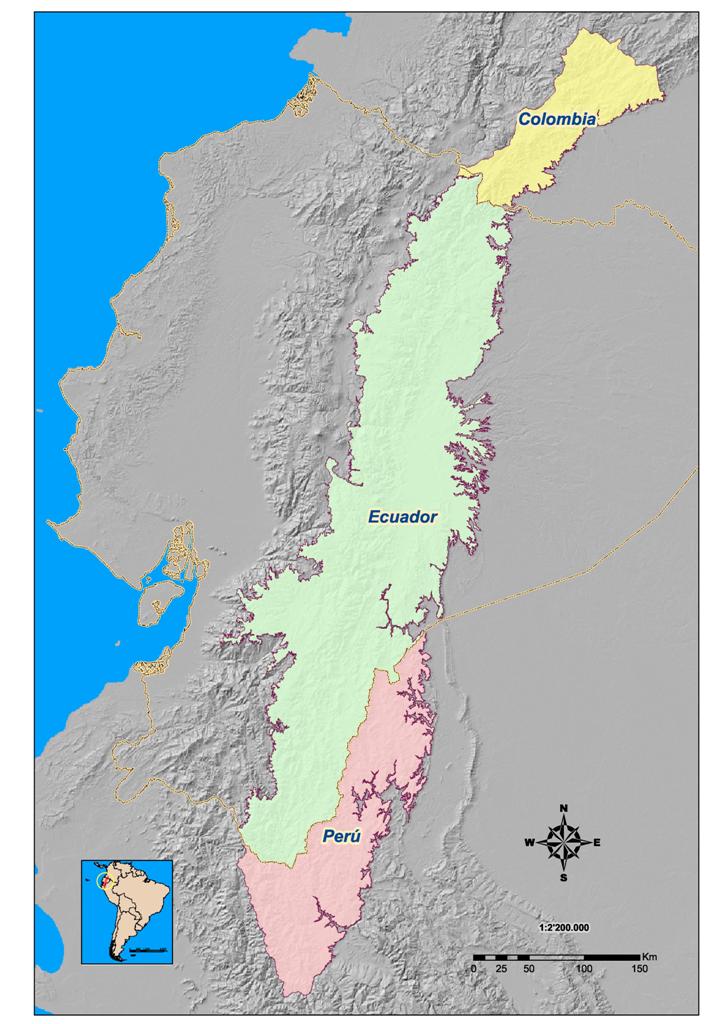
Figure 1. Location of the Eastern Cordillera in South America.

Distribution modeling

The process for distribution modeling relies on three main factors: (a) selection of species; (b) collection of presence points from museum specimens and herbaria records; and (c) generation of potential distribution maps for the selected species using GARP.
a. Selection of species
To understand the significance of a biodiversity index across geography, one needs context. Relationships between species and knowledge of lineages to which they belong provide that context (Erwing 1991).

We chose a suit of Andean-centered taxa (named Andean genera hereafter) that due to their intrinsic characteristics can be used as good descriptors of the diversity patterns of the Eastern Andean Ridge (Table 1). We selected nine Andean genera as biodiversity subrogates considering the following criteria: (1) their tempo and mode of radiation is related with the Andean uplift and the climatic shifts of the Pleistocene; (2) their overall distribution patterns present a high level of replacement within the environmental gradients; (3) several species of these genera present restricted distributions with a high level of endemism.

Among vascular plants we chose five genera that belong to the epiphytic or hemi-epiphytic life form. According to Jorgensen & León-Yanez (1999) more than a third of the plant species in the submontane and montane forest rainforest of Ecuador belong to these types of life form. Out of the total 2,110 native genera occurring in Ecuador the five selected are among the 20 most diverse genera with more than 20% of their listed species reported as endemics. This high level of diversity within these groups is related to the elevation of the Andes as well as to the climatic fluctuations during the Quaternary (Gentry 1982; Croat 1991; Luteyn 2002).

Among vertebrate groups we selected four Andean bird's genera (three hummingbird's genera, and one antpitta genus). We used bird species among others vertebrates because the available detailed distributional data, a well defined taxonomic classification and important literature dealing with their phylo-geographic patterns and ecology (Bleiweiss 1998a, b; Fjeldså & Krabbe 1990; Ridgely & Greenfield 2001; Rice 2005).

b. Collection of presence points

We collected species presence points from different datasets sources. Vascular plant specimen data were obtained from the Missouri Botanical Garden's VAST (Vascular Tropicos) nomenclatural database (MBG 2004), Herbarium specimens from the Herbarium of the Instituto Nacional de Ciencias (COL) in Colombia and the Catholic University Herbarium in Ecuador (QCA). Bird species data were obtained from the following databases: BirdLife International, Chicago Field Museum of Natural History (FMNH), Academy of Natural Sciences of Philadelphia (ANSP) and the Berkeley Museum of Natural History. Finally, additional data were obtained in private data bases (Juan Fernando Freile for Antpittas; Cal Dodson-Lorena Endara for orchid's records and James Luteyn's database stored at the New-York botanical Garden site (http://www.nybg.org) for Ericaceae).

Out of these databases, only those specimens whose collection localities were designated with geographic coordinates were selected (topographic maps 1:100.000 of the study area plus voucher level information were used to geo-reference all specimens) and from these, only the specimens identified at the species level by recognized experts of the group were considered for the next steps and further analysis.

After obtaining the presence records for each species of the selected Andean genera, the number of species for developing the models within GARP was further refined by choosing only those that had four or more geo-referenced specimens (named unique points of occurrence hereafter) in the biological databases.

The selection of a minimum sample size of four localities was based on conciliation between the data required to produce robust predictive models and the fact that most of the species had very few unique collection localities. However, other studies for not well explored areas have used as few as five and four records respectively (Anderson et al. 2002b; Anderson & Martínez-Meyer 2004).

c. Species Distribution Models (SDMs)

Generation of accurate and reliable distribution maps is based on the quality of the species occurrence points and on the selection and generation of a good set of predictive variables. According to previous studies (Leimbeck et al. 2004; Vargas et al. 2004; Luteyn 2002; Borchsenius 1997; Schuchmann et al. 2001; Heindl & Schuchmann 1998; Young et al. 2002; Jorgensen & León-Yanez 1999; Peralvo 2004; Boone & Krohn 2000) climatic and topographic variables (environmental variable hereafter) are the most important indirect predictors of present species assemblage within the Andes.

We selected a set of eleven environmental variables for plants and nine for birds considering the selected set as good indirect and direct descriptors of the patterns of abundance and distribution of the Andean biota (Table 2). The rationale of the selected set of environmental predictors is a balance between variables tested to influence species macro-distribution and the available information of environmental factors that can be translated into a continuous raster format within a regional geographic extent.

Each variable was created in raster format with 500 m resolution using the GIS software ArcGIS version 8.1 (Environmental Systems Research Institute, Redlands, California). The 500 m resolution was chosen as an intermediate point between the high resolution of the Digital Elevation Model (DEM) used to generate the elevation variable (90 m, see below) and the coarse resolution of the climatic variables. The elevation variable was generated using the DEM produced by the Radar Shuttle Topographic Mission (SRTM) at 90 m of resolution for the land areas of the world. The DEM for the study area was downloaded using the USGS Seamless Data Distribution System interface (http://seamless.usgs.gov), and then it was re-sampled to a 500 m resolution.

To refine the resolution of the crude climatic variables an interpolation method was applied to smooth the original resolution of 1 km2 to a resolution of 500 m using an Ordinary Kriging (Kolmogorov 1941) interpolator in the Geostatistical Analyst extension of ArcGIS. The interpolation was based on the original climate databases of the public domain Worldclime supported by the University of Berkley (http://www.biogeo.berkeley.edu/) for the period 1950-2000 (Hijmans et al. 2004) and the DEM.

Model building

Building ecological niche models to predict species ranges has been one of the main focuses over the last 10 years in landscape ecology and conservation biology (Peterson & Cohoon 1999). Special concern has been devoted to develop species ranges in poorly known regions where only presence points are available. Several analytical approaches have been applied to these challenges, varying from simple sets of rules based on overlays of environmental and species occurrences data creating a so-called "environmental envelop" (Krabbe et al. 1998) to sophisticated multivariate analyses such as mahalanobis distance (Cuesta et al. 2003) or logistic regression (Loiselle et al. 2003).

Among these methods, the Genetic Algorithm for Rule-Set Prediction (GARP, Stockwell & Noble 1992; Stockwell & Peters 1999) is being increasingly used in predictive models of species distributions. GARP is an artificial intelligence-based super-algorithm that works by combining sets of rules to build the most accurate prediction possible for the region being considered. GARP has been used, among other applications, to test different biogeographic theories (Anderson et al. 2002b), to evaluate colonization processes by invasive species and parasites (Peterson & Vieglais 2001; Peterson & Shaw 2003), and to assess the effects of climate change in the distribution of species (Peterson et al. 2001).

SDMs were developed using a PC desktop-implementation of the program GARP (http://www.lifemapper.org/desktopgarp/) following the optimization parameters suggested by Anderson et al. (2003), Loiselle et al. (2003), and Raxworthy et al. (2003). For species with more than 20 unique occurrence records, the records were randomly divided in two subsets: training points (75% of the species records) and testing points (25% of the points). For species with less than 20 occurrences, all the points were used as training points to develop the models.

In all cases, an algorithm convergence threshold of 0.01 was selected with 1,000 iterations as an upper limit for each run. Each model was set to perform 100 tasks in order to account for the elements of stochasticity inherent to genetic algorithms, which means GARP produces slightly different models in every run (Stockwell and Peterson 2002; Peralvo 2004).

Species distribution models were obtained based on the selection of the 10 best-fit models (the 10 runs best subset). The best subsets for each species were selected by means of Anderson et al. (2003) criteria for selecting optimal distribution models, which states that model performance follows an inverse relationship between omission and commission errors and that best models in general shows low omission errors and moderate commission indexes.

Thus, an omission threshold of 5% and a commission threshold of 50% of the distribution were set for each model. For species with less than 20 occurrence points, intrinsic measures of omission and commission were selected, whereas extrinsic measures were used for species with more than 20 occurrence points. Afterward, the 10 models included in the best subset were summed to create a composite map, and the final modeled range for each species was generated using the pixels that were predicted as part of the distribution in the 10 models. These models are referred to as the "potential distributions" of each species hereafter (Peralvo 2004).

SDMs evaluation

Model accuracy was evaluated based on a sensitivity analysis using extrinsic and intrinsic measures (Cumming 2000). Areas of predicted absence where the species has been recorded are regarded as omission errors (Type II error) or "false absence". Areas predicted as presence by the model but where the species has not been observed constitute commission errors (Type I error) or "false presence". False absence value is particularly useful because it measures the amount of unexplained variation in the data (number of residuals); the greater the values of false negatives, the more models are likely to be unrealistic.

Based on this criterion, the mean values of intrinsic omission error and extrinsic commission index were evaluated for the 10 models in the best subset together with the intrinsic overall accuracy and the percentage of non predicted area within the study area (Table 3). The intrinsic overall accuracy is a descriptive statistic derived from the confusion (error) matrix; where "a" and "d" represents the areas (number of pixels) correctly predicted as presence or absence. Conversely, "c" and "d" represents the omission and commission errors. This quantity ranges from 0 to 1.

Finally, for those target species for which a test dataset was available (n ≥ 20) a one tiled chi-squared test was performed. The significance of each model in the best subset was tested using a null hypothesis that no relationship existed between the test dataset and the predicted distributions.

Results

Species distribution models (SDMs)

We developed 138 SDMs (112 plant and 26 bird species) based on 1933 unique occurrence records for plant species and 517 points for bird species. The minimum number of records for a plant species was four (median = 11) and five (median = 18) for birds; the maximum number reached 80 unique records for a plant species (Cavendishia bracteata) and 54 for a bird (Grallaria rufula rufula). 71% and 54% of the modeled plant and bird species had less than 20 independent records.

Measures of model performance

a. Composite measures of performance

For those models with 20 or more points extrinsic performance measures (χ2) were almost always significant. All thirteen models for birds showed significant deviations from random predictions (χ2 = 7.31 - 71.52; p << 0.05). Thirty of 33 models for plants were highly significant (χ2 = 2.79 - 64.71; p << 0.05); the other 3 models had non-significant departure from the desired direction.

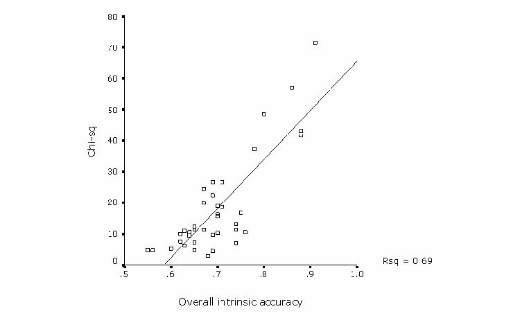
When comparing both plant and bird models with 20 or more points, a consistent trend was observed between intrinsic and extrinsic measures of overall model performance. The correlation analysis shows a highly significant relationship of both composite measures (r = 0.83; p < 0.01). The regression analysis explained the variation among both measures in 70% of the cases (Figure 2) showing a consistency on both indicators of model performance. Yet, variation in overall internal accuracy was minimal compared with a great variation in the extrinsic accuracy parameter. This may be related by the high susceptibility of the chi-square statistic towards the amount of test points and to the proportional extent of predicted presence. Thus, bird models in general had relative large number of test points which resulted in a high statistical power (Figure 3).

Figure 2. Regression analysis to test for a consistency between intrinsic and extrinsic measures of overall model performance

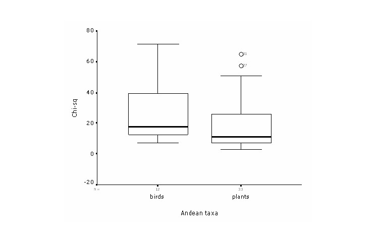
Figure 3. Boxplot comparing chi-square statistical power among birds and plant models.

b. Intrinsic omission and commission errors

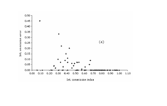
Within intrinsic values for omission index of the plants models did not track their corresponding commission values. Still, a modest negative correlation exists among these two variables (r = -0.58; p ( 0.01). The highest percent (93%) of the cases are clustered at omission values < 0.1, while the dispersion of the values within the commission axis is substantial with a great concentration of cases on the range between 0.75 and 1.0 (median = 0.79). A peculiar relationship is observed at the lower right side of the scatterplot, where all the cases with a commission value of over 0.70 had no training localities falling outside the predict area ((Figure 4a)).

Figure 4a. Intrinsic plots of omission error vs. commission index, for each of the (a) plant and (b) bird species.

This pattern might be explained by the strong relationship of the non-predicted area of the models with the internal commission index. Correlations between the two measures for the plant models were high (r = 0.89; p < 0.01), with highly significant regression (Rsq = 0.78; p < 0.001). All the cases with a commission index > 0.7 and a omission error of 0.0 have less than 20 occurrence points and, in the majority of the cases, had small geographic ranges (< 10.000 km2) and a mean overall accuracy of 0.51.
0.75) and the lowest omission error values (((Figure 4b)).

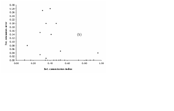
Figure 4b. Commission Index.

Correspondingly to the plant models, the latter pattern can be explained by contrasting the commission index with the percentage of area non-predicted of each model. A discrete positive correlation was observed among these two variables (r = 0.64; p < 0.01) suggesting that high commission values were partially related to a poor capacity of GARP on describing the realized niche of that particularly species. This analysis highlights the fact of 5 specific models that might have problems due to its high level of uncertainty. All these models have less than 20 training points and all but one (Eriocnemis luciani) present a restricted geographic extent (< 10,000 km2).

Discussion

Species ranges

Measures of model performance
Our results demonstrate the ability of GARP models to predict Andean species distributions over large geographic extents. GARP models are applicable to a variety of species with different ecological requirements and under different sample scenarios. Furthermore, predictions were tested in areas outside the spatial extent of the training data with high accuracy. Thus, ecological niche modelling is a promising tool for understanding species distributions in poorly known regions.
Our tests showed that internal overall accuracy measures help to evaluate the overall model performance. Yet, it fails as a measure of quality to discriminate among a suite of final GARP models. Although we demonstrated that GARP models can be used under different scenarios, the exploration of the model quality is rather complex, due to the high dispersion of the statistical measures between different scenarios. Models with more than 20 records showed a high dispersion of the chi-square statistic which makes it difficult to establish effective means for identifying the best models. According to Peterson et al. (2001) extrinsic model significance (χ2) probably varied among species in part due to the power afforded when varying sample sizes in the test data sets, and because of the relative extent of suitable habitat for each species. Conversely, in our study, the internal overall accuracy varied little among models. Stockwell & Peterson (2002b) and Anderson et al. (2003) also found that overall accuracy reached an apparent plateau with sample sizes of 20-50 localities. Thus, this measure helps to evaluate overall model performance but fails as a measure of quality to discriminate among a suite of final GARP models.
Likewise, the use of omission and commission errors may be useful for assessing overall model performance and to discriminate the best ones among several GARP outputs, because of the relative high sensitivity of the overall accuracy tests to sample sizes (Anderson et al. 2003). This quantities allowed us to evaluate models developed with no test points because patterns in intrinsic measures are repeated in the independent extrinsic ones; hence intrinsic measures hold potential for assessing model quality when all available data points are used for model construction.
The majority of the models for the widespread species combined low measures of omission with mid to fairly high levels of commission, and a fairly high overall intrinsic accuracy. These results concur with the findings of Peterson et al. (2002) and Anderson et al. (2003) who stated that in the best GARP models large areas are included as predicted presence (yielding high values in the commission index) in order to reduce omission to acceptable levels without overfitting the data.
The majority of the models for restricted range species showed extreme low omission values, extreme high commission values, and a relative mid overall intrinsic accuracy. The high commission values together with high number of cells where the algorithm could not define whether the species is present or absent, suggest a high degree of uncertainty in the produced models.
Consequently, the produced models overfitted the data by including most or all of the training points and small regions around them which mean GARP models included the core ecological distribution of that species, but excluded ecologically peripheral parts of possible distribution. According to Anderson et al. (2003) for these species (p.e., Grallaria ridgleyi; Ceratostema oellgardii), the best GARP models should minimize omission without increasing commission excessively (because pixels of predicted presence represent a small fraction of the study region) which was not the case for 35% of produced models.

Conclusions

a. Ecological modeling methods
Our results suggest that ecological niche modeling methods to predict the geographic distribution of Andean-centered taxa constitute a promising tool which allow evolutionary, biogeographic and conservation research based on data from specimens present in natural history collections. Predictive models of species distributions take advantage of the fact that museum and herbaria collections tend to be more biased in geographic space than in environmental space. Thus, predictive models allow estimating species' presence/absence patterns for large geographic areas, optimizing the use of existing presence-only datasets. The modeling system used in this study proved to be especially well suited for this application because in the majority of the cases its predictions were not affected by the spatial biases present in the biological databases.

Another advantage of using species distribution models as predictors of biodiversity patterns within the study area is the improvement in spatial resolution in relation to higher order surrogates such as vegetation types. Vegetation types assume a homogeneous distribution of an assemblage of species in each class, whereas species richness based on modeled distributions is likely to capture the heterogeneous nature of environmental variation more faithfully (Peralvo 2004). In this sense, predictive models work better than highly generalized and subjectively constructed estimations of species distributions, thus provide a systematic framework to evaluate distribution of species that can be quantitatively tested using independent data. Finally the selection of ecological meaningful taxa over a significant biogeographic unit allowed us to delineated, with a high accuracy level, areas of high endemism on the Eastern Cordillera.

The main limitations associated with predictive models are related to (1) the scarce quantity of independent species records, (2) the coarseness of the environmental predictors, and (3) the static nature of the modeling techniques derived from the necessary assumption of equilibrium. First, model accuracy tends to increase with sample size (e.g. Peterson et al. 2001; Stockwell & Peterson 2002a); however, the minimum sample size relays on the modeling method applied, the biology of the species, the environmental predictors used, and the environmental characteristics of the study area (Peterson et al. 2002). Nevertheless, setting an objectively threshold sample size requires testing the increment in predictive accuracy achieved at different sample sizes until a plateau in accuracy is reached (Anderson et al. 2002b; Stockwell & Peterson 2002a). Yet, this procedure requires relatively large sample sizes to test and train the models which are not the case for most rare and endemic species of the Andes. Consequently most studies that use biological collections as primary data sources have followed a rather arbitrary approach to the definition of minimum sample size requirements as in our case.

Second, the climatic variables used in this study are rather coarse, thus they might obscure specific environmental gradients which in turn are function of the species' fundamental niche. Finally, correlative modeling approaches do not allow the inclusion of dynamic processes that have important consequence in the distribution of species. As a result, models present commission and omission errors that reflect the uncertainty introduced by factors such as environmental and demographic stochasticity. In spite of these limitations, correlative models are appropriate when a preliminary assessment of the distribution patterns of species is required over large geographic areas, since at these scales bioclimatic factors play a fundamental role as controls of species distributions.

Acknowledgements

The reviews of R. Hofstede, J. Duivenvoorden, and S. Benítez helped greatly to improve the manuscript and are appreciated. We thank Frank van Manen, Laura Thomson, and Angela Parrado for their comments and language editing on early version of the manuscript. Our special gratitude to Juan Fernando Freile, Lorena Endara, James Luteyn, Kerem Boyla, Catherine Graham, Julio Betancourt, and Isidoro Sánchez for providing information and sharing their knowledge on the distribution of the selected taxa within the Eastern Cordillera. We would like to acknowledge all the institutions that made possible this research: The Nature Conservancy-Ecuador, EcoCiencia, Fundación Natura, Conservation International-Ecuador, Instituto Alexander von Humboldt, World Wildlife Fund-Colombia, Instituto Nacional de Ciencias-Universidad Nacional de Colombia, Birdlife International, Universidad de Cajamarca, Herbario Nacional (QCN-E), Corporación Ornitológica Ecuatoriana (CECIA), Chicago Field Museum of Natural History (FMNH), Academy of Natural Sciences of Philadelphia (ANSP), the Berkeley Museum of Natural History, and all the institutions that continuously provide information to the Tropicos Database stored at the Missouri Botanical Garden (MOBOT) web-browser search engine. This research was supported by The Nature Conservancy-Ecuador and the MacArthur foundation.

References

Anderson, R P., M. Laverde & A.T. Peterson. 2002a. Geographical distributions of spiny pocket mice in South America: Insights from predictive models. Global Ecology and Biogeography 11: 131-141.

Anderson, R.P., M. Laverde & A.T. Peterson. 2002b. Using niche-based GIS modeling to test geographic predictions of competitive exclusion and competitive release in South American pocket mice. Oikos 98: 3-16.

Anderson, R.P., D. Lew & A.T. Peterson. 2003. Evaluating predictive models of species' distributions: Criteria for selecting optimal models. Ecological Modeling 162: 211-232.

Anderson, R.P. & E. Martinez-Meyer. 2004. Modeling Species' distributions for preliminary conservation assessments: an implementation with the spiny pocket mice (Heteromys) of Ecuador. Biological Conservation 116: 167-179.

Avise, J.C. 2000. Phylogeography: the history and formation of species. Harvard University Press, Cambridge, Mass. USA.

Bleiweiss, R. 1998a. Tempo and mode of hummingbird evolution. Biological Journal of the Linnean Society 65: 63-76.

Bleiweiss, R. 1998b. Origin of hummingbird faunas. Biological Journal of the Linnean Society 65: 77-97.

Boone, R.B. & W.B. Krohn. 2000. Partitioning sources of variation in vertebrate species richness. Journal of Biogeography 27: 457-470.

Borchsenius, F. 1997. Patterns of plant species endemism in Ecuador. Biodiversity and Conservation 6: 379-399.

Croat T.B. 1991. A revision of Anthurium section Pachyneurium (Araceae). Annals of the Missouri Botanical Garden 78: 539-855.

Cuesta, F., M. Peralvo & F. van Manen. 2003. Andean bear habitat use in the Oyacachi River Basin, Ecuador. Ursus: 14: 198-209.

Cumming, G.S. 2000. Using between-model comparisons to fine-tune linear models of species ranges. Journal of Biogeography 27: 441-455.

Dinerstein, E., D.M. Olson, D.J. Graham, A.L. Webster, S.A. Primm, M.P. Bookbinder & G. Ledec. 1995. A conservation assessment of the terrestrial ecosystems of Latin America and the Caribbean. World Wildlife Fund and World Bank, Washington, DC.

Duellman, W. & E. Wild. 1993. Anuran amphibians from the Cordillera Huancabamba, Northern Peru: Systematics, ecology, and biogeography. Occasional papers of the Museum of Natural History. The University of Kansas, Lawrence 57: 1-53.

Erwing, T. 1991. An evolutionary basis for conservation strategies. Science 253: 750-752.

Fjeldså, J. 1995. Geographical patterns of neoendemic and older relict species of Andean forest birds: the significance of ecologically stable areas. in Churchill S.P., H. Balslev, E. Forero & J. L. Luteyn (Eds). Biodiversity and conservation of Neotropical Montane Forests - proceedings of the Neotropical Montane Forest Biodiversity and Conservation Symposium, the NYB, 21-26 June.1993. The Ney York botanical Garden. NY. Pp: 1-667.

Fjeldså, J. & N. Krabbe. 1990. Birds of the high Andes - A manual to the birds of the temperate zone of the Andes and Patagonia, South America. Zoological Museum - University of Copenhagen and Apollo Books. Svendborg.

Fjeldså, J., E. Lambin & B. Mertens. 1999. Correlation between endemism and local ecoclimatic stability documented by comparing Andean bird distributions and remotely sensed land surface data. I 22: 63-78.

García-Moreno, J., P. Arctander & J. Fjeldså. 1999. Strong Diversification at the treeline among Metallura hummingbirds. The Auk 116: 702-711.

Gentry, A. 1982. Neotropical Floristic Diversity: Phytogeographical connections between central and south america, pleistocene climatic fluctuations, or and accident of the Andean orogeny. Annals of the Missouri Botanical Garden 69: 557-593.

Guisan, A. 2002. Semiquantitative response models for predicting the spatial distribution of plant species. in Scott, J.M., P.J. Heglund & M.L. Morrison (Eds). Predicting species occurrences: issues of scale and accuracy. Pages 315-326 Island Press, Washington, D.C.

Guisan, A. & N.E. Zimmermann. 2000. Predictive habitat distribution models in ecology. Ecological Modeling 135:147-186.

Heindl, M. & K.L. Schuchmann. 1998. Biogeography, geographical variation and taxonomy of the Andean genus Metallura, Gould, 1847. Journal für Ornithologie 139: 425-473.

Hijmans, R.J., S. Cameron & J. Parra. 2004. WorldClim, version 1.2. A square kilometer resolution database of global terrestrial surface climate. Available at http://biogeo.berkeley.edu/

Http://www.biogeo.berkeley.edu/

Http://www.lifemapper.org/desktopgarp/

Http://www.nybg.org/bsci/res/lut2/

Http://seamless.usgs.gov/

Huston, M.A. 2002. Introductory Essay: Critical Issues for Improving Predictions. in Scott J.M., P.J. Heglund & M.L. Morrison (Eds). Predicting species occurrences: issues of scale and accuracy. Pages 7-21 Island Press, Washington, D.C.

Hutchinson, G.E. 1957. Concluding remarks. Cold Spring Harbor Symposium in Quantitative Biology 22: 415-427.

Jorgensen, P.M., D. Neill, & S. León-Yánez. 1999. Introduction. in Jorgensen P.M. & S. León-Yánez. (Eds). Catalogue of the vascular plants of Ecuador. Herbarium de la Universidad Católica del Ecuador, Herbarium of the Museo Ecuatoriano de Ciencias Naturales, and Department of Systematic Botany of Aahrus University. Pages 1-108 Missouri Botanical Garden Press, St. Louis.

Jorgensen, P.M. & S. Leon Yanez. (Eds). 1999. Catalogue of the vascular plants of Ecuador. Missouri Botanical Garden Press, St. Louis.

Jorgensen, P.M., C. Ulloa-Ulloa, J. Madsen &R. Valencia. 1995. A floristic analysis of the high Andes of Ecuador. in S.P. Churchill, H. Balslev, E. Forero & L. Luteyn (Eds). I. Pages 221-237 The New York Botanical Garden, New York, USA.

Kolmogorov, A.N. 1941. Interpolation and extrapolation of stationary random sequences. Isvestiia Akademii Nauk SSSR, Seriia Matematicheskiia 5: 3-14.

Krabbe, N., F. Skov, J. Fjeldså &I .K. Petersen. 1998. Avian diversity in the Ecuadorian Andes. Centre for Research on Cultural and Biological Diversity of Andean Rainforest (DIVA), 143 pp. DIVA Technical Report n°4. Denmark.

Leimbeck, R.M., R. Valencia & H. Balslev. 2004. Landscape diversity patterns and endemism of Araceae in Ecuador. Biodiversity and Conservation 13: 1755-1779.

Loiselle, B.A., C.A. Howell, C.H. Graham, J.M. Goerck, T. Brooks, K.G. Smith & P.H. Williams. 2003. Avoiding pitfalls of using species distribution models in conservation planning. Conservation Biology 17: 1591-1600.

Luteyn, J. 2002. Diversity, adaptation and endemism in neotropical Ericaceae: biogeographical patterns in the Vaccinieae. The Botanical Review 68: 55-87.

Missouri Botanical Garden (MBG). 2004. MOBOT - W3 TROPICOS.

Myers, N., R.A. Mittermeier, C.G. Mittermeier, G.A.B. da Fonseca & J. Kent. 2000. Biodiversity hotspots for conservation priorities. Nature 403: 853-858.

Peralvo, M.F. 2004. Identification of biodiversity conservation priorities using predictive modeling: An application for the tropical dry forests of western Ecuador and northern Peru. M.Sc. Thesis. University of Texas. Austin.

Peterson, A.T., Ball, L.G. & K.P. Cohoon. 2002. Predicting distributions of Mexican birds using ecological niche modeling methods. Ibis 144: 27-32.

Peterson, A.T. & P. Cohoon. 1999. Sensitivity of distributional prediction algorithms to geographic data completeness - Short communication -. Ecological Modelling 117: 159-164.

Peterson, A.T., V. Sanchez-Cordero, J. Soberon, J. Bartley, R.H. Buddemeier & A.G. Navarro-Siguenza. 2001. Effects of global climate change on geographic distributions of Mexican Cracidae. Ecological Modeling 144: 21-30.

Peterson, A.T. & J. Shaw. 2003. Lutzomyia vectors for cutaneous leishmaniasis in Southern Brazil: ecological niche models, predicted geographic distributions, and climate change effects. International Journal for Parasitology 33: 919-931.

Peterson, A.T. & D.A. Vieglais. 2001. Predicting species invasions using ecological niche modeling. BioScience 51: 363-371.

Raxworthy, C.J., E. Martinez-Meyer, N. Horning, R.A. Nussbaum, G.E. Schneider, M.A. Ortega-Huerta & A. Townsend-Peterson. 2003. Predicting distributions of known and unknown reptile species in Madagascar. Nature 426: 837-841.

Rice, N. 2005. Phylogenetic relationships of Antpitta genera (Passeriformes: Formicariidae). The Auk 122:673-683.

Ridgley, R. & P. Greenfield. 2001. The birds of Ecuador with the collaboration of M. Robbins and P. Coopmans. Cornell University Press. Ithaca, NY.

Schuchmann, K., A. Weller & I. Heynen. 2001. Systematics and biogeography of the Andean genus Eriocnemis (Aves: Trochilidae). Journal fuer Ornithologie 142: 433-481.

Stockwell, D.R.B. & A. T. Peterson. 2002a. Effects of sample size on accuracy of species distribution models. Ecological Modeling 148: 1-13.

Stockwell, D.R.B. & A. T. Peterson. 2002b. Controlling bias in biodiversity data. in Scott, J. M., P.J. Heglund & M.L. Morrison et al. (Eds). Predicting species occurrences: issues of scale and accuracy. Pages 537-545 Island Press, Washington D.C.

Stockwell, D.R.B. & D.P. Peters. 1999. The GARP modeling system: Problems and solutions to automated spatial prediction. International Journal of Geographic Information Systems 13: 143-158.

Stockwell, D.R.B. & I.R. Noble. 1992. Induction of sets of rules from animal distribution data: A robust and informative method of analysis. Mathematics and Computers in Simulation 33: 385-390.

Vargas, J.H., T. Consiglio, P.M. Jorgensen & T.B. Croat. 2004. Modelling distribution patterns in a species-rich plant genus, Anthurium (Araceae), in Ecuador. Diversity and Distribution 10: 211-216.

Williams, P.H., C. R. Margules & D.W. Hilbert. 2002. Data requirements and data sources for biodiversity priority area selection. Journal of Biosciences 27: 327-338.

World Wildlife Fund (WWF). 2001. Visión de la biodiversidad de los Andes del Norte. Santiago de Cali, Colombia (In Spanish).

Young, K., C. Ulloa Ulloa, J. Luteyn & S. Knapp. 2002. Plant Evolution and Endemism in Andean South America: An Introduction. The Botanical Review 68: 4-21.

Appendices: Tables

Table 1. Andean-centered taxa used as descriptors of the alpha diversity patterns on the Eastern Andean ridge (Table (a) refers to vascular plants and, table (b) to bird taxa).

(a)

Andean genera	Species recorded in Ecuador	Species recorded in Eastern cordillera	Percentage (%)	Endemic species recorded in Eastern cordillera	Percentage (%)
Anthurium	227	55	24.2	11	20.00
Lepanthes	287	194	67.6	118	60.82
Cavendishia	21	13	61.9	2	15.38
Ceratostema	28	28	100.0	26	92.86
Psammisia	26	17	65.4	5	29.41

(b)

Andean genera	Species recorded in Ecuador	Species recorded in CRO	Percentaje (%)	Endemic species recorded in CRO	Percentage (%)
Grallaria	15	12	80.00	2	16.67
Eriocnemis	7	5	71.43	2	40.00
Metallura	6	4	66.67	1	25.00
Coeligena	7	4	57.14	0	0.00

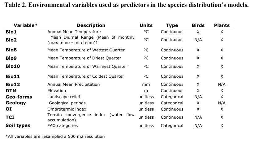
Table 2. Environmental variables used as predictors in the species distribution's models.

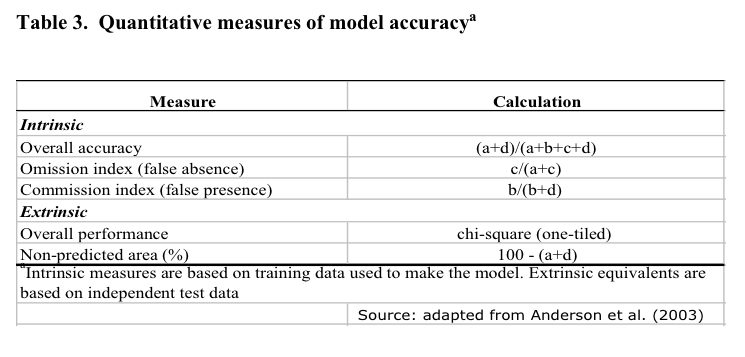
Table 3. Quantitative measures of model accuracy

-21-